US Treasury Yield Curve Analysis - Building the Full Fixed Income Pipeline from Scratch

Why I built this

I spent two years studying and working in quantitative finance: SOFR futures, SABR volatility surfaces, risk-neutral densities at a primary US Treasury dealer. But skills rust. Theory fades. The only way to reactivate real knowledge is to build something real. So I pulled six years of US Treasury yield data directly from the Federal Reserve and rebuilt the full yield curve analytics pipeline from scratch: historical visualization, bootstrapping, forward rates, and Nelson-Siegel fitting.

The macro story in five snapshots

The data covers January 2020 to June 2026 - one of the most dramatic rate cycles in modern history.

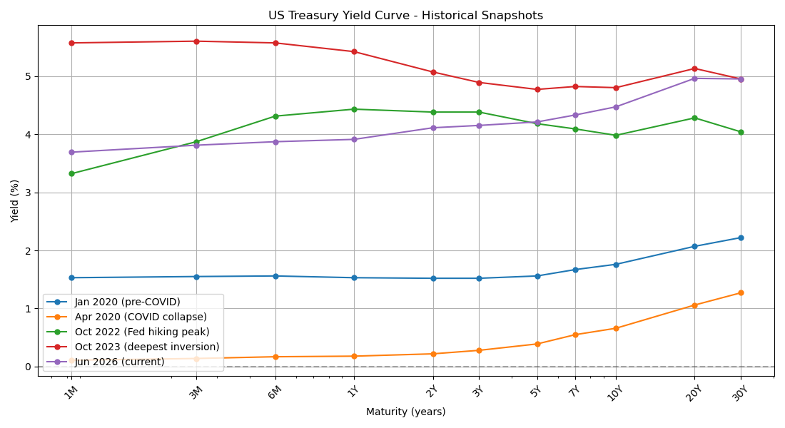
January 2020: the baseline. A normal upward-sloping curve. Short rates around 1.5%, long rates around 2.2%. Investors demanding more yield to lend for longer.

April 2020: COVID collapse. The Fed cut to zero overnight. The entire curve floored. Short end essentially at zero, 30Y barely above 1%. The most extreme monetary intervention since 2008.

October 2022: hiking cycle. The Fed raised rates aggressively to fight 8%+ inflation. The short end jumped to 4.3%. The long end barely moved, because long rates reflect expected future short rates, not current ones. The market didn't believe high rates would last forever.

October 2023: deepest inversion. The 2Y yielded more than the 10Y. The spread hit −0.93%, one of the deepest inversions since the early 1980s. Every US recession since the 1950s was preceded by an inversion. The market was pricing in eventual Fed cuts and economic slowdown.

June 2026: normalization. The spread is back to +0.35%. The curve is healing. Near-term cuts have been delivered, long rates have stabilized.

Bootstrapping the zero-coupon curve

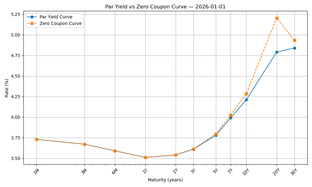
Par yields, the rates FRED publishes, are blended rates. A 10Y par yield of 4.21% doesn't mean every dollar you invest earns 4.21% for 10 years. It means the bond pays annual coupons, and those intermediate coupons get discounted at lower short-term rates. The par yield is an average across all those cash flows.

Zero-coupon rates strip that out. Each zero rate is the pure rate for a single cash flow at that exact maturity, no blending, no intermediate coupons. This is what you need to discount cash flows correctly, price derivatives, or build a risk-free rate for a DCF model.

Bootstrapping extracts zero rates iteratively. Start at the short end where par yield equals zero rate. Then for each longer maturity, discount the intermediate coupons using already-known zero rates, and solve algebraically for the unknown terminal zero rate. Work outward to 30 years.

The result: zero rates consistently exceed par yields on an upward-sloping curve. The 10Y zero rate (4.28%) sits above the 10Y par yield (4.21%). The 20Y shows the largest gap (+0.41%), amplifying a real kink in the January 2026 par curve caused by supply/demand dynamics specific to the 20Y Treasury.

The forward curve

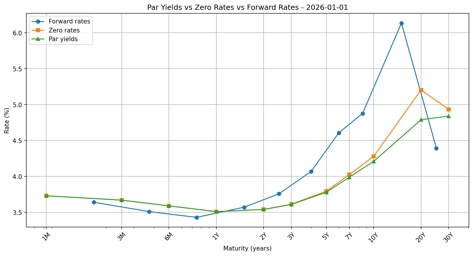
From the zero curve, you can extract forward rates, the rates the market implies for future periods. The 1Y1Y forward rate (the implied rate one year from now, for one year) is derived from:

f = ((1 + z₂)^T₂ / (1 + z₁)^T₁)^(1/(T₂-T₁)) - 1

The January 2026 forward curve told a clear story: near-term forwards were declining (market pricing in Fed cuts in 2026), medium-term forwards rose toward 4-5% (normalization), and long-dated forwards were elevated at 5-6% (term premium, fiscal uncertainty, inflation risk over decades).

The forward curve always sits above the zero curve which always sits above the par yield curve when the curve is upward sloping. Seeing all three together is the most complete picture of what the market is pricing.

Nelson-Siegel fitting

With 11 discrete data points, you can't evaluate yields at arbitrary maturities or compare curves across time with a single number. Nelson-Siegel solves this by fitting a smooth parametric curve using just four parameters:

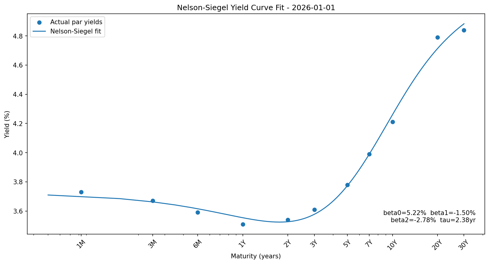
beta_0 = 5.22% - long-run level. Where the curve converges at infinite maturity.

beta_1 = −1.50% - slope. Negative means upward sloping; the short end starts 1.5% below the long-run level.

beta_2 = −2.78% - curvature. Negative means a downward hump concentrated around

tau = 2.38 years, capturing the residual distortion from the Fed hiking cycle.

tau = 2.38 years - the hump location. The curvature effect is most concentrated in the 2-3 year area.

Central banks and fixed income desks use Nelson-Siegel to track curve dynamics over time. Instead of saying "yields changed at 11 maturities in different directions," you say "the level rose 20bps, slope steepened 30bps." Interpretable and comparable.

What I relearned building this

First, the difference between par yields and zero rates is not theoretical, it's meaningful. Using a par yield to discount a single cash flow 20 years out introduces real error. The 20Y zero rate (5.20%) is 41bps above the 20Y par yield (4.79%). In a DCF model, that's significant.

Second, the forward curve is where the market's opinion lives. The par curve shows what things cost today. The forward curve shows what the market thinks will happen. Reading it is reading the market's forecast, imperfect, but the best aggregation of information available.

Third, Nelson-Siegel is simple and powerful in a way that's easy to underestimate. Four numbers fully describe a yield curve. That's not an approximation to be embarrassed about, it's a feature. Parsimony means you can compare January 2026 to October 2023 to April 2020 in a single table of four numbers per date. That's the kind of insight that's hard to get from raw data.

Links

GitHub: github.com/naumenko-analytics/treasury-yield-curve

LinkedIn: linkedin.com/in/mnaum